Weeks of September 20th

Sensitivity, CSV reading, and Pandas

What I did

• I found a website with lots of data science and machine learning questions that might be useful for interviews. I’ve done pretty well on some of them, but it’s also been a great way to see where I need to up-learn. For example, CVS reading and HTML parsing are things I’ve done before, but I couldn’t do a basic example if you woke me up in the middle of the night. That needs to change.

What I learned

• NLP
  • Lexical Analysis: Understanding the part of speech of a word
  • Syntactic Analysis: Analyzing words in a sentence for meaning
  • Semantic Analysis: Understanding exact meaning of words
  • Disclosure Integration: Understanding the context of the text (e.g. knowing you “he” refers to from the previous sentence)
  • Pragmatic Analysis: Understanding what a section of the text is actually about.
• Two downsides to measuring variance are that it has different dimensions than the original data (because you square it, often STD is more informative), and it is prone to outliers

\[Sensitivity = Recall = \frac{\text{True Positive}}{\text{(True Positive + Predicted Positive)}}\] \[Precision = \frac{\text{True Positive}}{\text{Predicted Positives}}\] \[F1 = \frac{2}{1/precision + 1/recall}\]

• How can you combat a dataset with a label imbalance so that your model performs well across all labels?
  • Perform subsampling of the dominant label and/or Perform oversampling of the least frequent label.
• Dealing with CSV’s recap.

  • better to just deal with it as a dataframe, especially if it has the first row as a column label

    with open(file) as f:
        df = pd.read_csv(f)
    

  • return the number of unique players in the year 1770. Column names are yearID and playerID

        df = df[df.yearID = '1970'].playerID.nunique()
    

  • If you don’t want to use pandas:

    players = defaultdict(set) #sets dictionary to fill blanks with 
    with open(file) as f:
        reader = csv.reader(f)
        columns = next(reader)
        for row in reader:
            # make a dict where key = year, val=set of player names
            players[int(row[0]).add(row[1])
        return len(players)
  
  

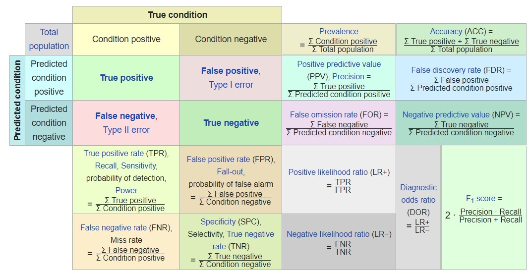
• ROC curve: (Receiver operating characteristic curve) is a graph showing the performance of a classification model at all classification thresholds. This curve plots true positive rate (TPR, sensitivity, recall, Power, probability of detection) and the false positive rate (FPR, type I error, fall-out). It shows the diagnostic ability of a binary classifier.

\[TPR = Recall = \frac{TP}{TP + FP} \\ FPR = \frac{FP}{TP + FP}\]

• The axes are from 0 to 1 with FPR on the x-axis and TPR on the y-axis. The axes represent the classification threshold. For example, if you’re predicting true or false, your classifier will spit out a value between 0 and 1 (usually by using a soft-max or a tanh activation function as the last layer). If you make the threshold = 0.8, the classifier will only predict true when it predicts a value >= 0.8. This threshold is not-so-much a tunable parameter as it is a chosen one. For example, if your classifier is supposed to determine if someone has cancer, maybe you want a threshold lower than 50% because the cost of making a wrong prediction could be dire. Or, maybe for a less consequential, extremely rare disease, you would want a threshold higher than 50%. This threshold is starting to sound bayesian, and reminds me of the fact that if a 99% TPR test predicts you have an extremely rare disease, it’s more likely a false positive than a true positive. Maybe I’ll do a separate post on this problem.
• The best possible option would be a point in the top left, (0,1). This would be 100% sensitivity (no false negatives) and 100% specificity (1 - FPR = specificity = all true positives).
• This means a perfect classifier has an AOC (area under the ROC curve) = 1, and the worst possible classifier would have an AOC = 0 (but, then you could just flip the predictions and have a perfect classifier instead)
• Curves above the y = x diagonal line represent better than random (good) classifiers.
  • The area under the curve of is a measure of the performance of a binary classifier across all possible classification thresholds.

Memorize this table from Wikipedia

What I will do next

• Since I never heard back from Sotheby’s for some reason, I’m going to switch my focus back to NLP and making my chatbot. I’m tempted to start over and do the whole thing again in PyTorch this time.

• Continue bayesian statistics

• Write IBM cover letters

• Drill that table posted above into my brain