The Dance of Forward Pass and Backprop

In order to implement a neural network, a solid understanding of Linear Algebra is needed for the forward pass, whereas vector calculus is needed for backpropagation. Neither action is particularly complicated, mathematically, however there are so many moving parts it is easy to get lost in the sea of similar sounding partial derivatives. Here, for my benefit, I’m going to walk through the math, as well as the full process of implementing the two function for an affine neural network with 2 hidden layers.

Feed Forward and Einstein Notation

There are enough capital sigmas in the world. I haven’t seen anyone use Einstein notation to represent the forward passes of a neural network. Perhaps this is because in practice one usually uses an activation function between each layer.

For a one layer (affine) neural network, the forward propagation is calculated as follows using Einstein notation:

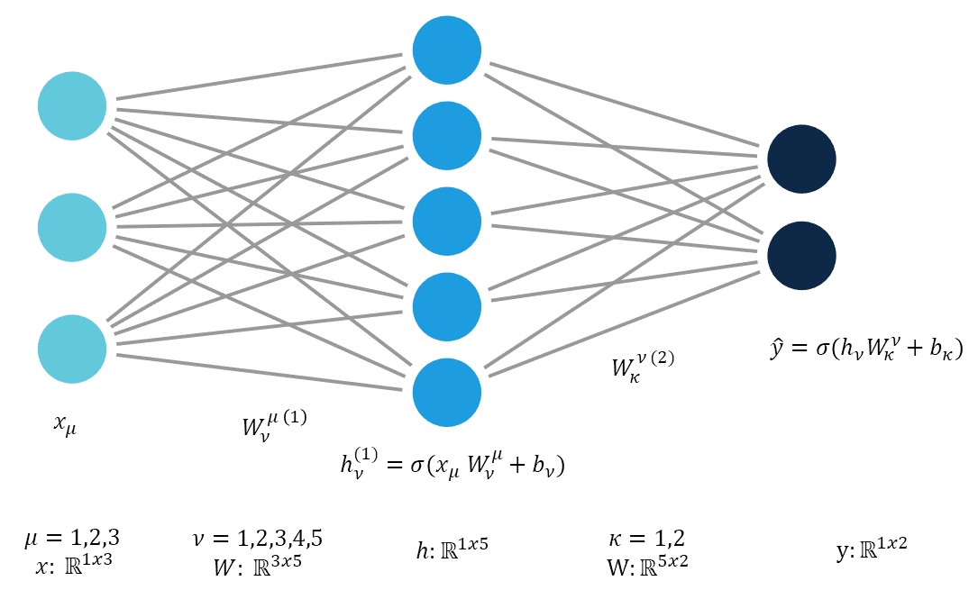
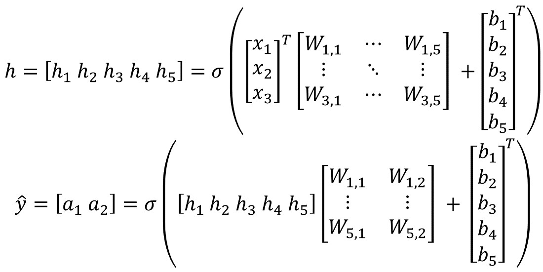
Recall that repeated indices are implicitly summed over. Explicitly, for one component of the hidden layer:

\[h_j = \sigma(w_{1j}x_1 + w_{2j}x_2 + w_{3j}x_3 + w_{4j}x_4 + w_{5j}x_5 + b_j) \\ = \sigma\Big(\sum_{i=1}^{i=5}w_{ij}x_{i} + b_j\Big)\]

And in vectorized form:

The process can be repeated ad-nauseam for networks with more layers.

Backpropagation

First, I will show the partial derivative chain rules, and then do it again, more explicitly with defined functions. For now, say your functional is:

\[\hat{y} = \sigma(g(f(x,y)))\]

This would be a network with inputs (x,y), two hidden layer (f and g), and an output with activation function sigma. Lets say the loss is the RMS loss. Thus,

\[L = \frac{1}{m} \sum (\hat{y} - y)^2\]

To see how much we need to shift the weights, we need to find the gradients for each layer. For the first partial derivative, we have:

\[\frac{\partial L}{\partial L} = 1\]

Trivial. Time for the next layer.

\[\frac{\partial \hat{y}}{\partial L} = \frac{\partial L}{\partial L}\frac{\partial \hat{y}}{\partial L}\]

It’s a little silly to write it this way, but I’m trying to demonstrate a pattern. Next layer:

\[\frac{\partial L}{\partial \sigma} = \frac{\partial L}{\partial \hat{y}} \frac{\partial \hat{y}}{\partial \sigma}\]

Next layer:

\[\frac{\partial L}{\partial g} = \frac{\partial L}{\partial \hat{y}} \frac{\partial \hat{y}}{\partial \sigma} \frac{\partial \sigma}{\partial g}\]

Next layer:

\[\frac{\partial L}{\partial f} = \frac{\partial L}{\partial \hat{y}} \frac{\partial \hat{y}}{\partial \sigma} \frac{\partial \sigma}{\partial g} \frac{\partial g}{\partial f}\]

The pattern should be clear. You multiply the gradient calculated in the previous layer by the partial the next layer w.r.t the previous layer.

Concrete Example

Let’s take the functional:

\[\hat{y} = \sigma(f(x)) \\ z = f(x) = W \cdot x + b\\ \sigma = \frac{1}{1+e^{-z}}\]

The sigmoid function is applied element-wise to the values calculated in \(f(x)\). I tried to indicate this by using z. As before:

\[Loss = L = \frac{1}{m}\sum(\hat{y} - y)^2 \\ \frac{\partial L}{\partial L} = 1\]

What we want to know how to shift the weights of the functions. We want to know \(\frac{\partial L}{\partial W}\), but it’ll take some work to get there. Now, explicitely,

\[\frac{\partial L}{\partial \hat{y}} = 2(\hat{y} - y )\]

So,

\[\frac{\partial L}{\partial \hat{y}} = \frac{\partial L}{\partial L}\frac{\partial L}{\partial \hat{y}} \\ = 1 \cdot 2(\hat{y} - y )\] \[\frac{\partial L}{\partial \sigma} = \frac{\partial L}{\partial \hat{y}} \frac{\partial \hat{y}}{\partial \sigma}\]

We already found the first part, but how about the second term in the chain? Well,

\[\frac{\partial \hat{y}}{\partial \sigma} = 1 \\ \implies \frac{\partial L}{\partial \sigma} = \frac{\partial L}{\partial \hat{y}} \frac{\partial \hat{y}}{\partial \sigma} \\ = 2(\hat{y} - y ) \cdot 1\]

Okay, now, let’s go a layer deeper.

\[\frac{\partial L}{\partial f} = \frac{\partial L}{\partial \hat{y}} \frac{\partial \hat{y}}{\partial \sigma} \frac{\partial \sigma}{\partial f}\]

So how about this next chain?

\[\frac{\partial \sigma}{\partial f} = \sigma(z)(1 - \sigma(z))\]

where z is the value of f(x). So,

\[\frac{\partial L}{\partial f} = 2(\hat{y} - y ) \cdot 1 \cdot \sigma(z)(1 - \sigma(z))\]

Now we’re up to the good part. The parameters we want to “wiggle” to change our network are the weights and biases (W and b). So,

\[\frac{\partial L}{\partial W} = \frac{\partial L}{\partial f} = \frac{\partial L}{\partial \hat{y}} \frac{\partial \hat{y}}{\partial \sigma} \frac{\partial \sigma}{\partial f} \frac{\partial f}{\partial W}\]

This last chain

\[\frac{\partial f}{\partial W} = x\]

So,

\[\frac{\partial L}{\partial W} = 2(\hat{y} - y ) \cdot 1 \cdot \sigma(z)(1 - \sigma(z)) \cdot x\]

And also,

\[\frac{\partial L}{\partial W} = \frac{\partial L}{\partial f} = \frac{\partial L}{\partial \hat{y}} \frac{\partial \hat{y}}{\partial \sigma} \frac{\partial \sigma}{\partial f} \frac{\partial f}{\partial b}\] \[\frac{\partial f}{\partial b} = 1\] \[\frac{\partial L}{\partial b} = 2(\hat{y} - y ) \cdot 1 \cdot \sigma(z)(1 - \sigma(z)) \cdot 1\]

This was just the process for a neural network with one hidden layer and a sigmoid activation function, but one can see how you could continue the process if you had more than one hidden layer. For example, after \(\frac{\partial L}{\partial f}\) you would chain \(\frac{\partial f}{\partial g}\) where g is the next hidden layer (f and g are swapped here with how I wrote it in the first part). If there were an activation function for this layer, which there often is, instead of \(\frac{\partial f}{\partial g}\), you would have to chain another \(\frac{\partial f}{\partial \sigma}\) first.

Here is basically a complete implimentation. To finish writing a classifier from scratch you’d need to initialize weights and the network structure. The full code for this can be found here.

def forward(self, X):
    """
    Performs the forward pass of the model.
    :param X: N x D array of training data. Each row is a D-dimensional point.
    :return: Predicted labels for the data in X, shape N x 1
              1-dimensional array of length N with classification scores.
    """
    assert self.W is not None, "weight matrix W is not initialized"
    # add a column of 1s to the data for the bias term
    batch_size, _ = X.shape
    X = np.concatenate((X, np.ones((batch_size, 1))), axis=1)
    # save the samples for the backward pass
    self.cache = X
    # output variable
    y = self.sigmoid( np.dot(X, self.W) ) # compute activation
    # cost = -(1/m)*(np.sum((Y*np.log(y)) + (1-Y) *np.log(1-y)))
    return y

def backward(self, y):
    """
    Performs the backward pass of the model.
    :param y: N x 1 array. The output of the forward pass.
    :return: Gradient of the model output (model output is y=sigma(X*W)) wrt W
    """
    assert self.cache is not None, "run a forward pass before the backward pass"

    # the gradient wrt W, dW
    # The data X is stored in self.cache.

    m = self.num_features
    X = self.cache

    z = np.dot(X, self.W)
    aL = self.sigmoid(z)
    dsig = self.sigmoid(z) * (1 - self.sigmoid(z))
    # db = (1/m) * np.sum(y-Y)
    dW = y * dsig * 2* (aL -y)
    return dW

def sigmoid(self, x):
        """
        Computes the ouput of the sigmoid function
        :param x: input of the sigmoid, np.array of any shape
        :return: output of the sigmoid with same shape as input vector x
        """
        out = 1 / (1 + np.exp(-1*x))
        return out