What I did

• Made a word cloud from my facebook messenger data. I realized that this was on my resume, but I never actually did it. It only took a day, since I already had the data and a solid understanding of its organization.
• I’ve been going through the Deep Learning practice exam as well as one I found from Stanford in preparation for my final next week.
• I took a break from studying by doing some coding challenges. I wrote linear regression (both with sklearn and from scratch), as well as calculating the Karl Pearson Correlation Coefficient (both with numpy and from scratch).

What I learned

• There’s some known bug in the facebook encoding scheme of the JSON file. This could be a reason why my chatbot was spitting out nonsense, though I suspect there are more issues with the chatbot project that I need to address. From what I found on the web, the JSON is encoded in uft-8, but gets decoded as latin-1, before being loaded as utf-8. To remedy this, reversed the process; I loaded the JSON, then went through line by line, encoding it in latin-1, then decoding it as utf-8 again.

def parse_obj(obj):
    for key in obj:
        if isinstance(obj[key], str):
            obj[key] = obj[key].encode('latin_1').decode('utf-8')
        elif isinstance(obj[key], list):
            obj[key] = list(map(lambda x: x if type(x) != str else x.encode('latin_1').decode('utf-8'), obj[key]))
        pass
    return obj

with open(sarah_json1) as f:
     fixed_json = json.load(f, object_hook=parse_obj)
     df = pd.json_normalize(fixed_json["messages"])

• I’m still facing issues with apostrophes. These don’t seem to be decoded correctly. I still have u'\u2019' (i.e. right single quotation marks) that show up. I can’t seem regex-replace them. This is particularly troublesome for this project because the word-cloud package interprets that symbol as cause to split the word in too. Thus, it’ll split a word like 'they're into they and re. The STOPWORDS package removes they from the cloud, but obviously re isn’t a word, but it is super common since they're is a common word. For now I’ve just added all the phonemes that follow apostrophes to the list of stop-words, but I need to fix this issue for the chatbot training data.

L1 vs L2 regularization

• L2 regularization is often referred to as weight decay, because:

where $\alpha$ is the learning rate, $\lambda$ is the regularization hyper-parameter, and J is the cost. Every iteration the weights are pushed closer to zero since your multiplying the weights by a number \(<1\). For L2, we have:

L1 regularization is just the same as above, but with an absolute value for the regularization term instead of a square. L1 is known as LASSO (least absolute shrinkage and selection operator), because it shrinks the less important features’ coefficients to zero. This is because for small values \(abs(w)\) is a much stiffer penalty than \(w^2\). Thus, L1 is thus a good choice when you have a ton of features.

Famous Network Architectures

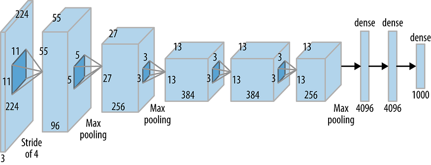
• AlexNet
  • CNN first used with huge success in predicting IMAGE-NET (1000 classes).
  • 5 convolutional layers, 3 fully-connected layers, ReLU activations
• VGGNet
  • CNN with a reduced number of parameters in the convolutional layers.
  • VGG16 refers to the fact that it has 16 total layers.
  • Each Conv kernel is 3x3 and each maxpool kernel is 2x2 with a stride of two.
  • The idea is that one 5 X 5 kernel is the equivalent of two 3 x 3 kernels (no padding and stride of 1 on an input of 5 x 5 x 1). Or one 7 X 7 can be replaced by three 3 X 3, or one 11 X 11 can be replaced by five 3 X 3 kernels.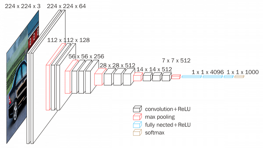
• ResNet
  • Solves the vanishing gradient problem by using “shortcut connections.”
  • These residuals blocks allow you to pass gradients back from deeper in the network.
  • Allows you to build deeper networks and still have it train better on the training set.
• Pearson Correlation coefficient:

Here, the top term is the covariance of x and y

and the bottom terms are just the standard deviation of x and of y.

What I will do next

• It might be more interesting to make word nets for each part of speech. I found some code I wrote earlier that uses word net to split the message corpus into parts of speech.